9.2: Infinite Series |
您所在的位置:网站首页 › math series › 9.2: Infinite Series |
9.2: Infinite Series
| Learning Objectives
Explain the meaning of the sum of an infinite series.
Calculate the sum of a geometric series.
Evaluate a telescoping series.
We have seen that a sequence is an ordered set of terms. If you add these terms together, you get a series. In this section we define an infinite series and show how series are related to sequences. We also define what it means for a series to converge or diverge. We introduce one of the most important types of series: the geometric series. We will use geometric series in the next chapter to write certain functions as polynomials with an infinite number of terms. This process is important because it allows us to evaluate, differentiate, and integrate complicated functions by using polynomials that are easier to handle. We also discuss the harmonic series, arguably the most interesting divergent series because it just fails to converge. Sums and SeriesAn infinite series is a sum of infinitely many terms and is written in the form \(\displaystyle \sum_{n=1}^∞a_n=a_1+a_2+a_3+⋯.\) But what does this mean? We cannot add an infinite number of terms in the same way we can add a finite number of terms. Instead, the value of an infinite series is defined in terms of the limit of partial sums. A partial sum of an infinite series is a finite sum of the form \(\displaystyle \sum_{n=1}^ka_n=a_1+a_2+a_3+⋯+a_k.\) To see how we use partial sums to evaluate infinite series, consider the following example. Suppose oil is seeping into a lake such that \( 1000\) gallons enters the lake the first week. During the second week, an additional \( 500\) gallons of oil enters the lake. The third week, \( 250\) more gallons enters the lake. Assume this pattern continues such that each week half as much oil enters the lake as did the previous week. If this continues forever, what can we say about the amount of oil in the lake? Will the amount of oil continue to get arbitrarily large, or is it possible that it approaches some finite amount? To answer this question, we look at the amount of oil in the lake after \( k\) weeks. Letting \( S_k\) denote the amount of oil in the lake (measured in thousands of gallons) after \( k\) weeks, we see that \( S_1=1\) \( S_2=1+0.5=1+\frac{1}{2}\) \( S_3=1+0.5+0.25=1+\frac{1}{2}+\frac{1}{4}\) \( S_4=1+0.5+0.25+0.125=1+\frac{1}{2}+\frac{1}{4}+\frac{1}{8}\) \( S_5=1+0.5+0.25+0.125+0.0625=1+\frac{1}{2}+\frac{1}{4}+\frac{1}{8}+\frac{1}{16}.\) Looking at this pattern, we see that the amount of oil in the lake (in thousands of gallons) after \( k\) weeks is \[ S_k=1+\frac{1}{2}+\frac{1}{4}+\frac{1}{8}+\frac{1}{16}+⋯+\frac{1}{2^{k−1}}=\sum_{n=1}^k\left(\frac{1}{2}\right)^{n−1}. \nonumber \] We are interested in what happens as \( k→∞.\) Symbolically, the amount of oil in the lake as \( k→∞\) is given by the infinite series \[\sum_{n=1}^∞\left(\frac{1}{2}\right)^{n−1}=1+\frac{1}{2}+\frac{1}{4}+\frac{1}{8}+\frac{1}{16}+⋯. \nonumber \] At the same time, as \( k→∞\), the amount of oil in the lake can be calculated by evaluating \(\displaystyle \lim_{k→∞}S_k\). Therefore, the behavior of the infinite series can be determined by looking at the behavior of the sequence of partial sums \( {S_k}\). If the sequence of partial sums \( {S_k}\) converges, we say that the infinite series converges, and its sum is given by \(\displaystyle \lim_{k→∞}S_k\). If the sequence \( {S_k}\) diverges, we say the infinite series diverges. We now turn our attention to determining the limit of this sequence \( {S_k}\). First, simplifying some of these partial sums, we see that \( S_1=1\) \( S_2=1+\frac{1}{2}=\frac{3}{2}\) \( S_3=1+\frac{1}{2}+\frac{1}{4}=\frac{7}{4}\) \( S_4=1+\frac{1}{2}+\frac{1}{4}+\frac{1}{8}=\frac{15}{8}\) \( S_5=1+\frac{1}{2}+\frac{1}{4}+\frac{1}{8}+\frac{1}{16}=\frac{31}{16}.\) Plotting some of these values in Figure, it appears that the sequence \( {S_k}\) could be approaching 2. 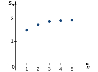 Figure \(\PageIndex{1}\): The graph shows the sequence of partial sums \({S_k}\). It appears that the sequence is approaching the value \(2\).
Let’s look for more convincing evidence. In the following table, we list the values of \(S_k\) for several values of \(k\). \( k\) 5 10 15 20 \( S_k\) 1.9375 1.998 1.999939 1.999998These data supply more evidence suggesting that the sequence \({S_k}\) converges to \(2\). Later we will provide an analytic argument that can be used to prove that \(\displaystyle \lim_{k→∞}S_k=2\). For now, we rely on the numerical and graphical data to convince ourselves that the sequence of partial sums does actually converge to \(2\). Since this sequence of partial sums converges to \(2\), we say the infinite series converges to \(2\) and write \[ \sum_{n=1}^∞\left(\frac{1}{2}\right)^{n−1}=2.\nonumber \] Returning to the question about the oil in the lake, since this infinite series converges to \(2\), we conclude that the amount of oil in the lake will get arbitrarily close to \(2000\) gallons as the amount of time gets sufficiently large. This series is an example of a geometric series. We discuss geometric series in more detail later in this section. First, we summarize what it means for an infinite series to converge. DefinitionAn infinite series is an expression of the form \[\sum_{n=1}^∞a_n=a_1+a_2+a_3+⋯. \nonumber \] For each positive integer \(k\), the sum \[S_k=\sum_{n=1}^ka_n=a_1+a_2+a_3+⋯+a_k \nonumber \] is called the \(k^{\text{th}}\) partial sum of the infinite series. The partial sums form a sequence \({S_k}\). If the sequence of partial sums converges to a real number \(S\), the infinite series converges. If we can describe the convergence of a series to \(S\), we call \(S\) the sum of the series, and we write \[\sum_{n=1}^∞a_n=S. \nonumber \] If the sequence of partial sums diverges, we have the divergence of a series. Note that the index for a series need not begin with \(n=1\) but can begin with any value. For example, the series \[\sum_{n=1}^∞\left(\frac{1}{2}\right)^{n−1} \nonumber \] can also be written as \[\sum_{n=0}^∞\left(\frac{1}{2}\right)^n\; \text{or}\; \sum_{n=5}^∞\left(\frac{1}{2}\right)^{n−5}. \nonumber \] Often it is convenient for the index to begin at \(1\), so if for some reason it begins at a different value, we can re-index by making a change of variables. For example, consider the series \[ \sum_{n=2}^∞\frac{1}{n^2}. \nonumber \] By introducing the variable \(m=n−1\), so that \(n=m+1,\) we can rewrite the series as \[ \sum_{m=1}^∞\frac{1}{(m+1)^2}. \nonumber \] Example \(\PageIndex{1}\): Evaluating Limits of Sequences of Partial SumsFor each of the following series, use the sequence of partial sums to determine whether the series converges or diverges. \(\displaystyle \sum_{n=1}^∞\frac{n}{n+1}\) \(\displaystyle \sum_{n=1}^∞(−1)^n\) \(\displaystyle \sum_{n=1}^∞\frac{1}{n(n+1)}\)Solution a. The sequence of partial sums \({S_k}\) satisfies \(S_1=\dfrac{1}{2}\) \(S_2=\dfrac{1}{2}+\dfrac{2}{3}\) \(S_3=\dfrac{1}{2}+\dfrac{2}{3}+\dfrac{3}{4}\) \(S_4=\dfrac{1}{2}+\dfrac{2}{3}+\dfrac{3}{4}+\dfrac{4}{5}\). Notice that each term added is greater than \(1/2\). As a result, we see that \(S_1=\dfrac{1}{2}\) \(S_2=\dfrac{1}{2}+\dfrac{2}{3}>\dfrac{1}{2}+\dfrac{1}{2}=2\left(\dfrac{1}{2}\right)\) \(S_3=\dfrac{1}{2}+\dfrac{2}{3}+\dfrac{3}{4}>\dfrac{1}{2}+\dfrac{1}{2}+\dfrac{1}{2}=3\left(\dfrac{1}{2}\right)\) \(S_4=\dfrac{1}{2}+\dfrac{2}{3}+\dfrac{3}{4}+\dfrac{4}{5}>\dfrac{1}{2}+\dfrac{1}{2}+\dfrac{1}{2}+\dfrac{1}{2}=4\left(\dfrac{1}{2}\right).\) From this pattern we can see that \(S_k>k\left(\frac{1}{2}\right)\) for every integer \(k\). Therefore, \({S_k}\) is unbounded and consequently, diverges. Therefore, the infinite series \(\displaystyle \sum^∞_{n=1}\frac{n}{n+1}\) diverges. b. The sequence of partial sums \({S_k}\) satisfies \(S_1=−1\) \(S_2=−1+1=0\) \(S_3=−1+1−1=−1\) \(S_4=−1+1−1+1=0.\) From this pattern we can see the sequence of partial sums is \[{S_k}={−1,0,−1,0,…}. \nonumber \] Since this sequence diverges, the infinite series \(\displaystyle \sum^∞_{n=1}(−1)^n\) diverges. c. The sequence of partial sums \( {S_k}\) satisfies \( S_1=\dfrac{1}{1⋅2}=\dfrac{1}{2}\) \( S_2=\dfrac{1}{1⋅2}+\dfrac{1}{2⋅3}=\dfrac{1}{2}+\dfrac{1}{6}=\dfrac{2}{3}\) \( S_3=\dfrac{1}{1⋅2}+\dfrac{1}{2⋅3}+\dfrac{1}{3⋅4}=\dfrac{1}{2}+\dfrac{1}{6}+\dfrac{1}{12}=\dfrac{3}{4}\) \( S_4=\dfrac{1}{1⋅2}+\dfrac{1}{2⋅3}+\dfrac{1}{3⋅4}+\dfrac{1}{4⋅5}=\dfrac{4}{5}\) \( S_5=\dfrac{1}{1⋅2}+\dfrac{1}{2⋅3}+\dfrac{1}{3⋅4}+\dfrac{1}{4⋅5}+\dfrac{1}{5⋅6}=\dfrac{5}{6}.\) From this pattern, we can see that the \( k^{\text{th}}\) partial sum is given by the explicit formula \[ S_k=\frac{k}{k+1} \nonumber \]. Since \( k/(k+1)→1,\) we conclude that the sequence of partial sums converges, and therefore the infinite series converges to \( 1\). We have \[ \sum_{n=1}^∞\frac{1}{n(n+1)}=1. \nonumber \] Exercise \(\PageIndex{1}\)Determine whether the series \(\displaystyle \sum^∞_{n=1}\frac{n+1}{n}\) converges or diverges. HintLook at the sequence of partial sums. AnswerThe series diverges because the \( k^{\text{th}}\) partial sum \( S_k>k\). The Harmonic SeriesA useful series to know about is the harmonic series. The harmonic series is defined as \[\sum_{n=1}^∞\frac{1}{n}=1+\frac{1}{2}+\frac{1}{3}+\frac{1}{4}+⋯. \nonumber \] This series is interesting because it diverges, but it diverges very slowly. By this we mean that the terms in the sequence of partial sums \( {S_k}\) approach infinity, but do so very slowly. We will show that the series diverges, but first we illustrate the slow growth of the terms in the sequence \( {S_k}\) in the following table. \( k\) 10 100 1000 10,00 100,000 1,000,000 \( S_k\) 2.92897 5.18738 7.48547 9.78761 12.09015 14.39273Even after \( 1,000,000\) terms, the partial sum is still relatively small. From this table, it is not clear that this series actually diverges. However, we can show analytically that the sequence of partial sums diverges, and therefore the series diverges. To show that the sequence of partial sums diverges, we show that the sequence of partial sums is unbounded. We begin by writing the first several partial sums: \( S_1=1\) \( S_2=1+\dfrac{1}{2}\) \( S_3=1+\dfrac{1}{2}+\dfrac{1}{3}\) \( S_4=1+\dfrac{1}{2}+\dfrac{1}{3}+\dfrac{1}{4}\). Notice that for the last two terms in \( S_4\), \[ \frac{1}{3}+\frac{1}{4}>\frac{1}{4}+\frac{1}{4} \nonumber \] Therefore, we conclude that \[ S_4>1+\frac{1}{2}+\left(\frac{1}{4}+\frac{1}{4}\right)=1+\frac{1}{2}+\frac{1}{2}=1+2\left(\frac{1}{2}\right). \nonumber \] Using the same idea for \( S_8\), we see that \(\displaystyle S_8=1+\frac{1}{2}+\frac{1}{3}+\frac{1}{4}+\frac{1}{5}+\frac{1}{6}+\frac{1}{7}+\frac{1}{8}>1+\frac{1}{2}+\left(\frac{1}{4}+\frac{1}{4}\right)+\left(\frac{1}{8}+\frac{1}{8}+\frac{1}{8}+\frac{1}{8}\right)=1+\frac{1}{2}+\frac{1}{2}+\frac{1}{2}=1+3\left(\frac{1}{2}\right)\). From this pattern, we see that \( S_1=1, S_2=1+1/2, S_4>1+2(1/2),\) and \( S_8>1+3(1/2)\). More generally, it can be shown that \( S_{2^j}>1+j(1/2)\) for all \( j>1\). Since \( 1+j(1/2)→∞,\) we conclude that the sequence \( {S_k}\) is unbounded and therefore diverges. In the previous section, we stated that convergent sequences are bounded. Consequently, since \( {S_k}\) is unbounded, it diverges. Thus, the harmonic series diverges. Algebraic Properties of Convergent SeriesSince the sum of a convergent infinite series is defined as a limit of a sequence, the algebraic properties for series listed below follow directly from the algebraic properties for sequences. Note \(\PageIndex{1}\): Algebraic Properties of Convergent SeriesLet \(\displaystyle \sum_{n=1}^∞ a_n\) and \(\displaystyle \sum_{n=1}^∞ b_n\) be convergent series. Then the following algebraic properties hold. i. The series \(\displaystyle \sum_{n=1}^∞(a_n+b_n)\) converges, and \(\displaystyle \sum^∞_{n=1}(a_n+b_n)=\sum^∞_{n=1}a_n+\sum^∞_{n=1}b_n.\) (Sum Rule) ii. The series \(\displaystyle \sum_{n=1}^∞(a_n−b_n)\) converges, and \(\displaystyle \sum^∞_{n=1}(a_n−b_n)=\sum^∞_{n=1}a_n−\sum^∞_{n=1}b_n.\) (Difference Rule) iii. For any real number \( c\), the series \(\displaystyle \sum_{n=1}^∞ca_n\) converges, and \(\displaystyle \sum^∞_{n=1}ca_n=c\sum^∞_{n=1}a_n\). (Constant Multiple Rule) Example \( \PageIndex{2}\): Using Algebraic Properties of Convergent SeriesEvaluate \(\displaystyle \sum_{n=1}^∞\left[\frac{3}{n(n+1)}+\left(\frac{1}{2}\right)^{n−2}\right].\) Solution We showed earlier that \[ \sum_{n=1}^∞\frac{1}{n(n+1)} = 1 \nonumber \] and \[ \sum_{n=1}^∞\left(\frac{1}{2}\right)^{n−1}=2. \nonumber \] Since both of those series converge, we can apply the properties of Note \(\PageIndex{1}\) to evaluate \[\sum_{n=1}^∞\left[\frac{3}{n(n+1)}+\left(\frac{1}{2}\right)^{n−2}\right]. \nonumber \] Using the sum rule, write \(\displaystyle \sum_{n=1}^∞\left[\frac{3}{n(n+1)}+\left(\frac{1}{2}\right)^{n−2}\right]=\sum_{n=1}^∞\frac{3}{n(n+1)}+\sum_{n=1}^∞\left(\frac{1}{2}\right)^{n−2}.\) Then, using the constant multiple rule and the sums above, we can conclude that \(\displaystyle \sum^∞_{n=1}\frac{3}{n(n+1)}+\sum^∞_{n=1}\left(\frac{1}{2}\right)^{n−2}=3\sum^∞_{n=1}\frac{1}{n(n+1)}+\left(\frac{1}{2}\right)^{−1}\sum^∞_{n=1}\left(\frac{1}{2}\right)^{n−1}=3(1)+\left(\frac{1}{2}\right)^{−1}(2)=3+2(2)=7.\) Exercise \(\PageIndex{2}\)Evaluate \(\displaystyle \sum^∞_{n=1}\frac{5}{2^{n−1}}\). HintRewrite as \(\displaystyle \sum^∞_{n=1}5\left(\frac{1}{2}\right)^{n−1}\). Answer10 Geometric SeriesA geometric series is any series that we can write in the form \[ a+ar+ar^2+ar^3+⋯=\sum_{n=1}^∞ar^{n−1}. \nonumber \] Because the ratio of each term in this series to the previous term is r, the number r is called the ratio. We refer to a as the initial term because it is the first term in the series. For example, the series \[\sum_{n=1}^∞\left(\frac{1}{2}\right)^{n−1}=1+\frac{1}{2}+\frac{1}{4}+\frac{1}{8}+⋯ \nonumber \] is a geometric series with initial term \( a=1\) and ratio \( r=1/2\). In general, when does a geometric series converge? Consider the geometric series \[\sum_{n=1}^∞ar^{n−1} \nonumber \] when \( a>0\). Its sequence of partial sums \( {S_k}\) is given by \[S_k=\sum_{n=1}^kar^{n−1}=a+ar+ar^2+⋯+ar^{k−1}. \nonumber \] Consider the case when \( r=1.\) In that case, \[S_k=a+a(1)+a(1)^2+⋯+a(1)^{k−1}=ak. \nonumber \] Since \( a>0\), we know \( ak→∞\) as \( k→∞\). Therefore, the sequence of partial sums is unbounded and thus diverges. Consequently, the infinite series diverges for \( r=1\). For \( r≠1\), to find the limit of \( {S_k}\), multiply Equation by \( 1−r\). Doing so, we see that \[ (1−r)S_k=a(1−r)(1+r+r^2+r^3+⋯+r^{k−1})=a[(1+r+r^2+r^3+⋯+r^{k−1})−(r+r^2+r^3+⋯+r^k)]=a(1−r^k). \nonumber \] All the other terms cancel out. Therefore, \( S_k=\dfrac{a(1−r^k)}{1−r}\) for \( r≠1\). From our discussion in the previous section, we know that the geometric sequence \( r^k→0\) if \( |r|1\) or \( r=±1\). Therefore, for \( |r| |
【本文地址】
今日新闻 |
点击排行 |
|
推荐新闻 |
图片新闻 |
|
专题文章 |